The piezo tutorial “Quasi-static actuators” describes applications where dynamics (acceleration, damping) can be neglected. However, in many applications, dynamics play an important role and have to be taken into account in the design process. The tutorial gives an introduction to dynamic applications. A simplified model is presented, to analyze and estimate the behavior of the dynamic system both for sinusoidal and for step excitation. Finally, the aspects of heat dissipation are presented.
Dynamic Behaviour of Piezoelectric Actuators
What is a dynamic application?
In a dynamic application, the dynamic forces (inertia or mass multiplied by acceleration) and damping forces (force depending on speed) are not negligible. As a result, the system cannot be modeled by simple linear equations, but by differential equations.
The limit between a static and a dynamic application depends on many parameters. If a mechanical resonance is present at less than three times the operating frequency, then the application is dynamic. Fast driving signals (steps) also call for a dynamic analysis.
Simple dynamic model
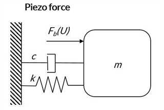
In a static application, a piezoelectric actuator can be modeled as a spring, with a characteristic that can be offset by an electrical field. For a dynamic application, this model has to be expanded to include at least the damping and mass of the moving part (piezo + load). The piezo effect can be modeled as an external force, proportional to the voltage, acting on the load.
In this approach, the system is equivalent to a damped harmonic oscillator, driven by the piezoelectric force. This means that for a given driving force (i.e. voltage amplitude) with an increasing frequency, the amplitude of the displacement will increase up to the mechanical resonance, then decrease. Phase will change from 0 to 180°.The amplification factor due to resonance can be substantial, leading to increased stress on the piezo element. Therefore, in most cases the excitation signal will need to be reduced around resonance.
A simple dynamic model for piezoelectric multilayer actuators
Limitations
It is important to know what limits the performance of the piezoelectric actuator in the application. Limitations can be of three types:
- Voltage-related. Actuators are designed for a certain voltage range. Operation outside of that range is not recommended as it could cause electrical failure (arcing) or accelerated ageing.
- Stress-related. Actuators are specified for a certain stress range. For example, the plate stacks are recommended in the range +10 to +80MPa, although in extreme cases they can be used in the range -5 to +150MPa. Tensile stress can result in a mechanical damage while compressive stress leads to a degradation of the poling.
- Temperature-related. Although the normal operating range of piezoelectric multilayer actuators is very wide (for example 4mK to 470K/200°C for one of our standard products), self-heating is a concern for high frequency operation.
Since stress and self-heating are directly related to frequency, it is important to understand the dynamics of a system in order to validate the design of the piezoelectric element.
The Mason Model, Definition and Identification of the Dynamic Parameters
The Mason model
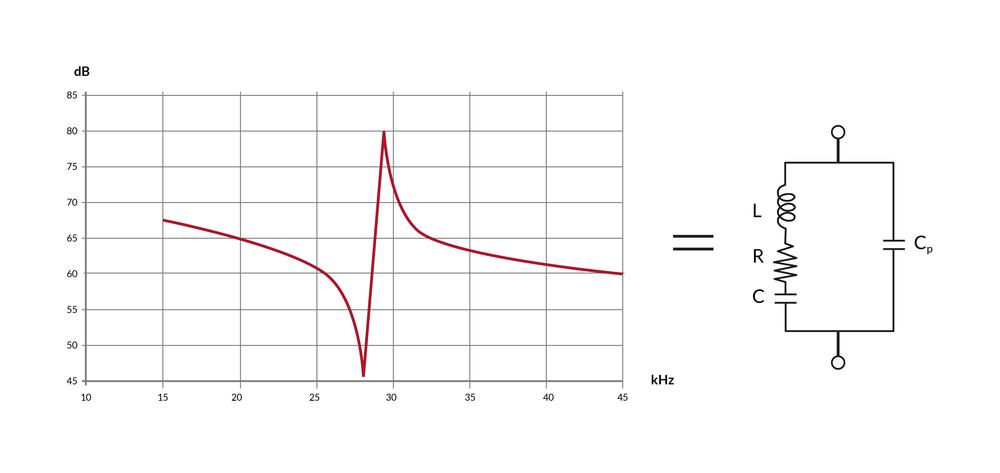
Since the dynamic system can be modeled using differential equations, there are a number of different ways to model, analyze and estimate the behavior. A very common method is to use a Mason model (similar to Butterworth-van Dyke equivalent circuit), which is an electrical equivalent of the equations of motion including the piezo effect.
The equation of motion can be written:
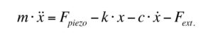
The equation of motion
An electrical equivalent can be written:
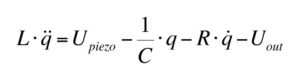
Mason’s electric equivalent of the equation of motion
This type of model can be extended to include more resonances, however in practice this is only useful for systems operating in a very wide frequency range.
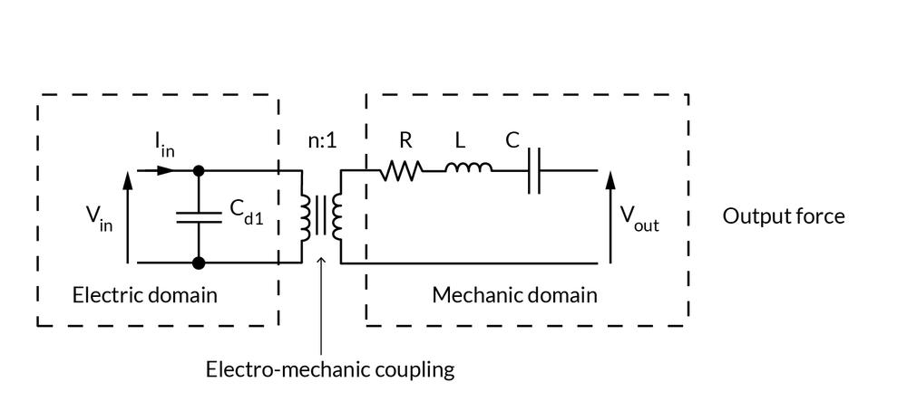
Electro-mechanical coupling (piezo effect)
Description of the parameters
Vin is the voltage applied on the piezo. This voltage is used to charge the electrical capacitance, and this way, generate a piezo force on the system.
The electro-mechanical coupling n describes the piezoelectric effect, i.e. the conversion of electrical energy to mechanical energy.
The system mass m is equivalent to an inductance L. This parameter describes the inertia of the system. A high value will drag the resonance frequency down.
The system stiffness k is equivalent to the inverse of a capacitance C. A high value of the stiffness (i.e. low value of the equivalent capacitance) will increase the resonance frequency of the system.
The system damping c is equivalent to a resistance R. Damping depends mostly on the materials used. High damping will lead to a slower but more stable step response. In an oscillating application, damping will reduce the overshoot around resonance but will lead to increased heat dissipation.
Identification of the parameters
There are different ways of identifying the parameters of a dynamic system.
A common method is to measure the impedance spectrum of the piezoelectric element. Because of the electro-mechanical coupling, mechanical resonances are visible on the spectrum and can be modeled.
However, this method has two major drawbacks. First, it is only applicable for small signals and dynamic parameters tend to change for large signal. Second, it can only identify four parameters, therefore one is missing to relate the electrical equivalent to the mechanical domain.
Methods based on large signal excitation and direct measurement of mechanical parameters (typically displacement) provide more accurate models. There are different methods; the most common one is to measure amplitude and phase of the displacement for an electrical excitation at different frequencies (Bode plot). Parameters can also be identified based on the step response of the system.
Graph showing the impedance spectrum
Resonance Frequency of Multilayer Actuator Stacks
It is sometimes useful to estimate the frequency response of a multilayer stack in free conditions. The task is not straightforward, but it is usually possible to generate good estimates of the first resonance. Depending on the configuration, this first resonance can be a thickness mode or a width/radial/hoop mode.
For high stacks (“elongated rod” assumption), the first resonance will be a thickness mode. The first thickness resonance Ft can be estimated using the formula:
Ft=N3/H
With H the height of the stack, and N3 a material constant. Experimentally, N3 differs slightly from the catalog value, which is obtained on monolayer components of a specific geometry. We recommend using the typical values below:
Typical N3 value for multilayer stacks, free-free conditions:
NCE51 and NCE51F: 1200 Hz.m
NCE46: 1400 Hz.m
For example on the multilayer actuator stack NAC2003-H12, the first thickness resonance in free conditions will be 100kHz (typical value).
The thickness resonance is divided by 2 if the actuator is in blocked-free conditions. Attached load (mass) further reduces the value.
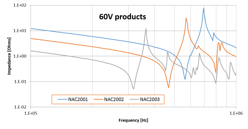
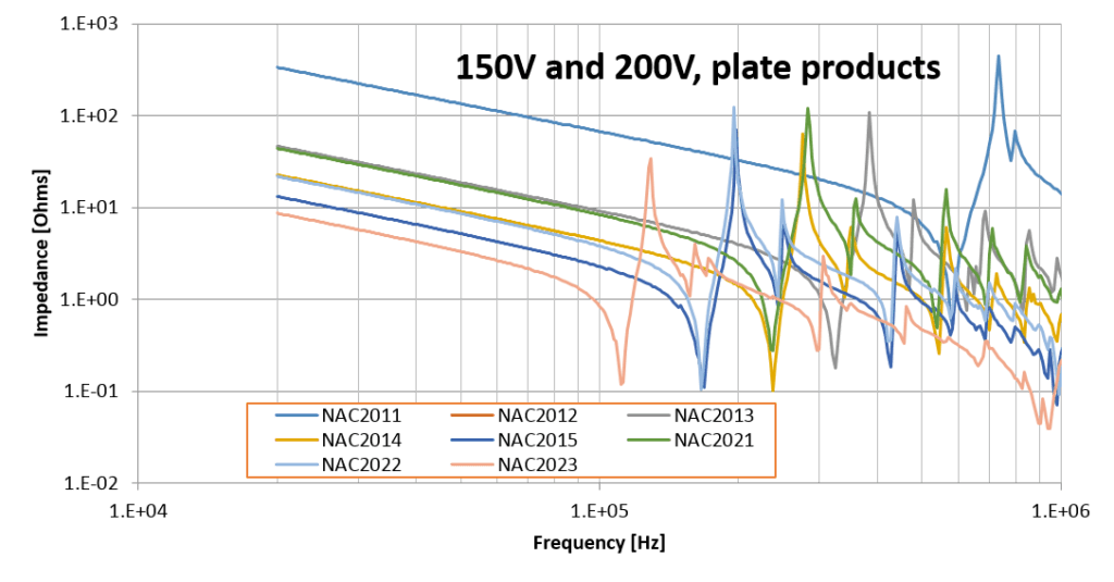
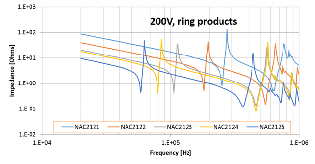
For short and wide stacks (“thin plate” assumption), a width/radial/hoop resonance will be the first one to occur. This type of resonance depends on the cross-section of the actuator. The graphs below illustrate the frequency response of a selection of CTS’s range of multilayer single element actuators, for which the first radial resonance can be identified.
If a thickness resonance and a radial resonance are close to each other, they tend to interact. The case is not ideal (neither an “elongated rod” nor a “thin plate”), so the mode shapes are more complex and frequencies can vary.
Learn more about our multilayer products
Important Calculations: Sinusoidal Operation
Current
Off-resonance, a piezoelectric actuator is mostly capacitive, so the supply current can be estimated using the simplified formula below.
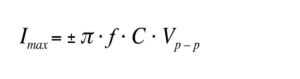
Equation to estimate the supply current
With:
f: operating frequency
C: apparent piezo capacitance
Vp-p: peak to peak voltage
Note that the apparent capacitance increases with the amplitude of the input signal. At full amplitude, current draw can be 40% higher than calculated using the small signal capacitance.
Around resonance, in the case of an actuator providing high coupling, the actuator deviates from the capacitive behaviour; therefore, the other parameters in the model have to be taken into account.
Dynamic force
In dynamic mode, inertial forces due to the fast acceleration of a mass are dependent on frequency as seen in the formula below.
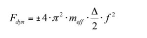
Equation to estimate the dynamic stress
With:
f: operating frequency
meff: equivalent moving mass
Δ: peak to peak displacement
Calculations – stress limit
This equation can be used as a first approach to estimate the dynamic stress on the actuator due to the acceleration. In more complex cases, for example in the case of high damping, it is recommended to use a more detailed model for the estimation of the maximum stress.
Important Calculations: Step Response
Charging time
For the generation of steps, it is not physically possible to charge a piezo actuator instantly. Instead, in most cases the waveform will be trapezoidal, with a given charging time. Charging time will depend mainly on the slew rate or current capability of the driver and the capacitance of the piezo element.
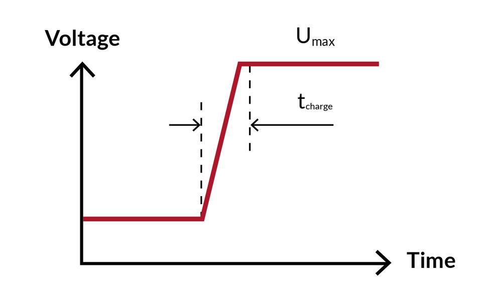
Graph showing the charging time in the relationship between voltage and time
Oscillations and optimal step response
Depending on the charging time and the mechanical resonance frequency of the system f0, the system will oscillate more or less.
For a long charging time (tcharge >> 1/f0), the system is close to quasi-static conditions and there will be very little oscillation.
For a short charging time (tcharge < 1/f0), the system will experience a shock that will lead to the largest oscillations.
Near the resonance period (tcharge ≈ 1/f0), the system can react fast with minimum oscillation. This is sometimes referred to as a “tuned step”. This method requires a precise knowledge or identification of the dynamic characteristics of the system, which is not always straightforward, in particular in the case of variable operating conditions (typically a changing mass load).
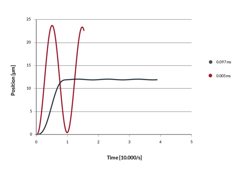
This can be illustrated on these simulation results based on a multilayer plate stack in blocked-free configuration, acting on a mass load of 20g (damping is reduced to illustrate the oscillations). Such a system has an undamped resonance period of 1/f0=0.097ms. Relatively large oscillations are generated for tcharge = 0.07ms and tcharge = 0.12ms while a “tuned step” (tcharge = 0.097ms) provides a fast and stable positioning.
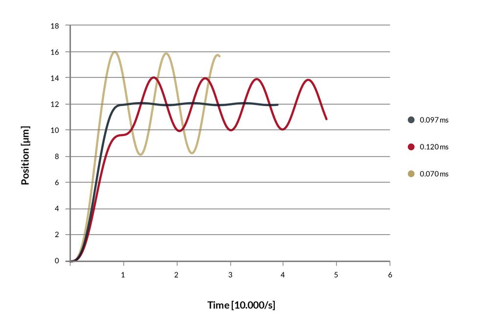
Graph showing oscillations and optimal step response
Fastest step response
For a very short charging time (tcharge << 1/f0) the actuator can reach the target position after 1/(3.f0). That is the fastest possible movement; however, it should be noted that it generates very large oscillations (illustration below, without damping).
Furthermore, the current requirements are much higher than with a “tuned step”. For the two examples below, there is a factor 20 difference in peak current. Also, acceleration and therefore stress is higher (factor 6).
Graph showing the fastest step response vs. tuned step
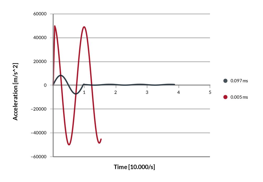
Graph showing the acceleration under fastest step response and tuned step
Heat Dissipation
Self-heating, i.e. heat generation within the piezoelectric actuator due to electrical and mechanical losses, is a major concern for high frequency applications. Properties (capacitance, stroke, etc.) will evolve with temperature, with the risk of unstable performance, increase stress and even degradation of the actuator.
Average power dissipation
In sinusoidal operation, the average power dissipation in a piezoelectric actuator can be estimated using the formula below:
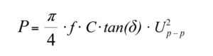
Equation to estimate the average power dissipation in a piezoelectric multilayer actuator
Where:
Where:tan (δ) = apparent dielectric dissipation factor
C = apparent PZT actuator capacitance [Farad]
Up-p = peak-peak drive voltage [V]
f = operating frequency [Hz]
Note that on datasheets, C and tan(δ) are specified for small signals. At 3kV/mm, the product C*tan(δ) is typically 7 to 10 times higher.
Surface and core temperature
The knowledge of the average dissipation in the actuator is not sufficient to determine its temperature. It is necessary to know the geometry and thermal properties of the system, such as:
Surfaces and materials in contact for the evaluation of thermal conduction
Free surfaces, fluid type (air, oil) and flow for the evaluation of natural or forced convection
For vacuum applications, the presence of radiating surfaces.
Generally speaking, small samples are easier to cool down because of the higher surface to volume ratio. Hard-doped ceramic is also advantageous at equivalent performance. Here are some indicative examples of temperature rise in natural convection conditions:
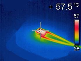
Image showing a small sample, hard-doped ceramic 3*3*2mm, 200V, lying on a ceramic plate in ambient conditions, operated at 2kHz, full amplitude heating-up by +30°C
A large sample, soft-doped ceramic (10*10*50mm, 200V), in the same ambient conditions, operated at 40Hz, full amplitude will heat-up by +70°C.
The best approach is to monitor temperature using a thermocouple, and eventually run thermal simulations during the design phase. The fact that large components can have a significant temperature gradient (core temperature is higher than surface temperature) should also be taken into account.
Thermal inertia
Piezoceramic material has a rather low heat conductivity but rather high heat capacity . Therefore, actuators tend to have a long thermal inertia, which means that they need a significant amount of time to heat-up or cool down. It is not uncommon that it takes one hour for a large stack to reach steady state.
If an actuator is operated for a short time at high power, it might not heat-up significantly. However, if that burst is repeated periodically, the long-term average power should be considered.